I wrote a very simple and user-friendly method, that I called ddeint, to solve delay differential equations (DDEs) in Python, using the ODE solving capabilities of the Python package Scipy. As usual the code is available at the end of the post :).
Example 1 : Sine
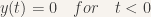
I start with an example whose exact solution is known so that I can check that the algorithm works as expected. We consider the following equation:


The trick here is that 
from pylab import *

model = lambda Y,t : Y(t - 3*pi/2) # Model
tt = linspace(0,50,10000) # Time start, end, and number of points/steps
g=sin # Expression of Y(t) before the integration interval
yy = ddeint(model,g,tt) # Solving

# PLOTTING
fig,ax=subplots(1)
ax.plot(tt,yy,c='r',label="$y(t)$")
ax.plot(tt,sin(tt),c='b',label="$sin(t)$")
ax.set_ylim(ymax=2) # make room for the legend
ax.legend()
show()

The resulting plot compares our solution (red) with the exact solution (blue). See how our result eventually detaches itself from the actual solution as a consequence of many successive approximations ? As DDEs tend to create chaotic behaviors, you can expect the error to explode very fast. As I am no DDE expert, I would recommend checking for convergence in all cases, i.e. increasing the time resolution and see how it affects the result. Keep in mind that the past values of Y(t) are computed by interpolating the values of Y found at the previous integration points, so the more points you ask for, the more precise your result.
Example 2 : Delayed negative feedback
You can select the parameters of your model at integration time, like in Scipy’s ODE and odeint. As an example, imagine a product with degradation rate r, and whose production rate is negatively linked to the quantity of this same product at the time (t-d):
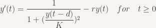
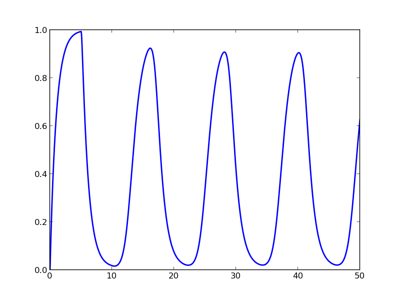
We have three parameters that we can choose freely. For K = 0.1, d = 5, r = 1, we obtain oscillations !
from pylab import *

# MODEL, WITH UNKNOWN PARAMETERS
model = lambda Y,t,k,d,r :  1/(1+(Y(t-d)/k)**2) - r*Y(t)

# HISTORY
g = lambda t:0

# SOLVING
tt = linspace(0,50,10000)
yy = ddeint(model,g,tt,fargs=( 0.1 , 5 , 1 )) # K = 0.1, d = 5, r = 1

# PLOTTING
fig,ax=subplots(1)
ax.plot(tt,yy,lw=2)
show()
Example 3 : Lotka-Volterra system with delay
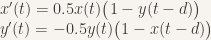
The variable Y can be a vector, which means that you can solve DDE systems of several variables. Here is a version of the famous Lotka-Volterra two-variables system, where we introduce some delay d. For d=0 we find the solution of a classical Lotka-Volterra system, and for d non-nul, the system undergoes an important amplification:

from pylab import *

def model(Y,t,d):
    x,y = Y(t)
    xd,yd = Y(t-d)
    return array([0.5*x*(1-yd), -0.5*y*(1-xd)])

g = lambda t : array([1,2])
tt = linspace(2,30,20000)
fig,ax=subplots(1)

for d in [0, 0.2]:
    yy = ddeint(model,g,tt,fargs=(d,))
    # WE PLOT X AGAINST Y
    ax.plot(yy[:,0],yy[:,1],lw=2,label='delay = %.01f'%d)

ax.legend()
show()

Example 4 : A DDE with varying delay
This time the delay depends on the value of Y(t) !

from pylab import *
model = lambda Y,t:  -Y(t-3*cos(Y(t))**2)
tt = linspace(0,30,2000)
yy = ddeint(model, lambda t:1, tt)
fig,ax=subplots(1)
ax.plot(tt,yy,lw=2)
show()

Code
Explanations
The code is written on top of Scipy’s ‘ode’ (ordinary differential equation) class, which accepts differential equations under the form
model(Y,t) = ” expression of Y'(t) ”
where 

For our needs, we need the input 


To this end, I first implemented a class (ddeVar) of variables/functions which can be called at any time 


Such variables need to be updated every time a new value of
Ok, here you are for the code
You will find the code and all the examples as an IPython notebook HERE (if you are a scientific pythonist and you don’t know about the IPython notebook, you are really missing something !). Just change the extension to .ipynb to be able to open it. In case you just asked for the code:
# REQUIRES PACKAGES Numpy AND Scipy INSTALLED
import numpy as np
import scipy.integrate
import scipy.interpolate

class ddeVar:
    """ special function-like variables for the integration of DDEs """


    def __init__(self,g,tc=0):
        """ g(t) = expression of Y(t) for t<tc """

        self.g = g
        self.tc= tc
        # We must fill the interpolator with 2 points minimum
        self.itpr = scipy.interpolate.interp1d(
            np.array([tc-1,tc]), # X
            np.array([self.g(tc),self.g(tc)]).T, # Y
            kind='linear', bounds_error=False,
            fill_value = self.g(tc))


    def update(self,t,Y):
        """ Add one new (ti,yi) to the interpolator """

        self.itpr.x = np.hstack([self.itpr.x, [t]])
        Y2 = Y if (Y.size==1) else np.array([Y]).T
        self.itpr.y = np.hstack([self.itpr.y, Y2])
        self.itpr.fill_value = Y


    def __call__(self,t=0):
        """ Y(t) will return the instance's value at time t """

        return (self.g(t) if (t<=self.tc) else self.itpr(t))


class dde(scipy.integrate.ode):
    """ Overwrites a few functions of scipy.integrate.ode"""


    def __init__(self,f,jac=None):

        def f2(t,y,args):
            return f(self.Y,t,*args)
        scipy.integrate.ode.__init__(self,f2,jac)
        self.set_f_params(None)


    def integrate(self, t, step=0, relax=0):

        scipy.integrate.ode.integrate(self,t,step,relax)
        self.Y.update(self.t,self.y)
        return self.y


    def set_initial_value(self,Y):

        self.Y = Y #!!! Y will be modified during integration
        scipy.integrate.ode.set_initial_value(self, Y(Y.tc), Y.tc)


def ddeint(func,g,tt,fargs=None):
    """ similar to scipy.integrate.odeint. Solves the DDE system
        defined by func at the times tt with 'history function' g
        and potential additional arguments for the model, fargs
    """

    dde_ = dde(func)
    dde_.set_initial_value(ddeVar(g,tt[0]))
    dde_.set_f_params(fargs if fargs else [])
    return np.array([g(tt[0])]+[dde_.integrate(dde_.t + dt)
                                 for dt in np.diff(tt)])
Other implementations
If you need a faster or more reliable implementation, have a look at the packages pyDDE and pydelay, which seem both very serious but are less friendly in their syntax.
